Gain vs. HV
Rationale
This measurement aims to find the voltage to apply to the PMT or DEgg to reach a gain of 1E7. The PMT comes with a nominal voltage from Hamamatsu, which is used as an anchor for four scan points in low voltage.
We record waveforms at SPE level, at ~10% occupancy, integrate the charge in a predefined signal window in the waveform. Applying a factor of 1/R, where R is the termination of the PMT base, a histogram is constructed. It contains a pedestal peak, corresponding to waveforms without any signal, includes a contribution from badly amplified photoelectrons, as well as a single-photo-electron (SPE) peak. There also might be a small contribution from double PE events.
Setup
The measurement is done in the 2D scan box, with the motors in rest position, shining perpendicular light onto the middle of the photocathode. The PMT is mounted in the scan box to the holder shown in figure Fig. 12.
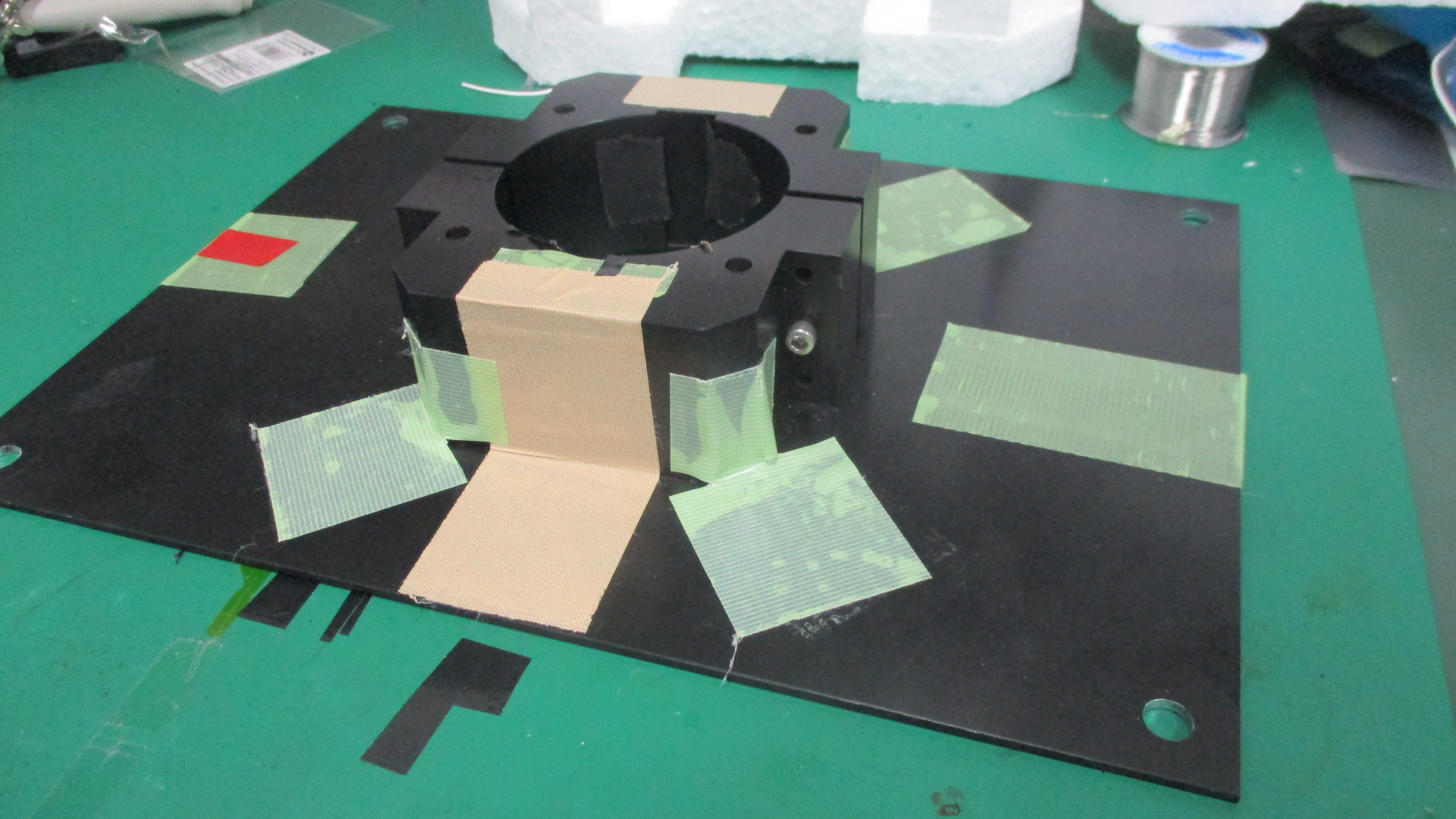
Fig. 12 The PMT holder for the DEgg 8inch PMTs for the scanbox.
When mounting the PMT into the holder, please do it as given in Fig. 13.
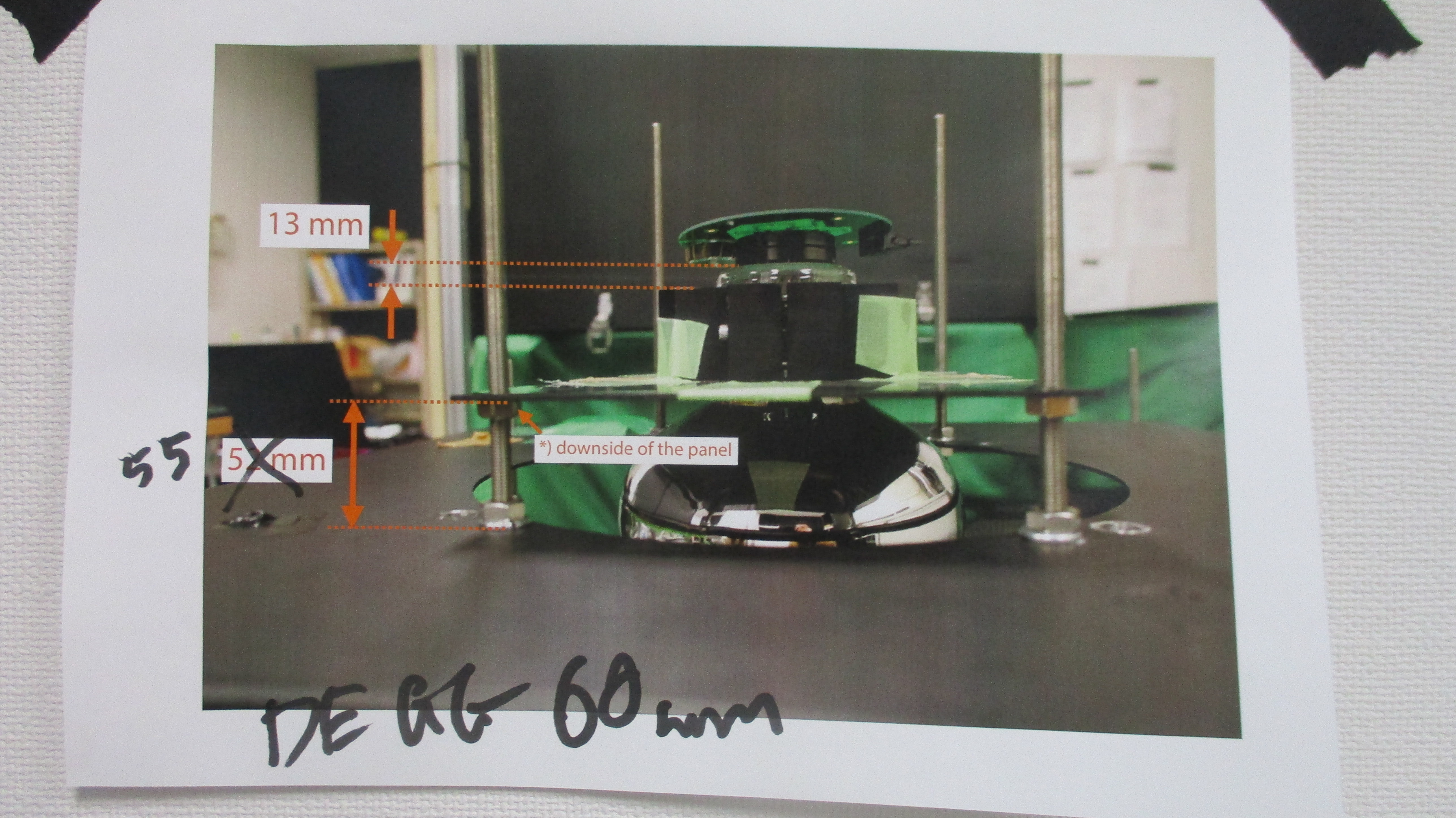
Fig. 13 Mounting geometry of a DEgg PMT into the 2D scan box. The distance between the upper side of the holder and the glass bottom of the PMT should be 13mm. The distance between the base plate in the scan box and the lower side of the PMT mount, should be 55mm when mounting a PMT, and 60mm when mounting a Degg.
After mounting the PMT into the 2D scan box, a HV board needs to be assigned to the PMT. That board should always be the same for each measurement of that PMT. The boards have two connectors, one for supplying bias and control voltage, and one SMA connector for the signal output.
The DAQ settings are the ones listed in Ayumis
sheet. The purpose of these settings is
to ensure datataking at SPE level. Since the optical setup is very
sensitive towards small changes, take the laser intensity setting as more of a
guide and not as an exact value.
Running the DAQ
The data acquisition is controlled by a jupyter notebook, it is located at:
/home/icecube/measurements/daq/notebooks/gain_calibration.ipynb
The oscilloscope is read out via ethernet, the voltage is also controlled via ethernet. The first thing the notebook does is extracting the nominal voltage value for a gain of 1E7 given by Hamamatsu. It then constructs a list of low voltage values around, which will be used to scan the gain.
The notebook automatically sets the low voltage value to the HV board and then records 10000 waveforms for every scan value.
After manually running the analysis scripts as described in the next section, the appropriate control voltage is extracted. The notebook then records 40000 waveforms at 1E7 gain, allowing for more precise determination of gain, SPE resolution, and peak-to-valley ratio.
Analysis
There is a Readme for the usage of the analysis scripts. It is located at:
/home/icecube/measurements/analysis/workspace/gain/README
First, check that the signal and baseline gates are aligned correctly by running:
/home/icecube/measurements/analysis/workspace/gain/tools/waveform_checks.py
If the gates look fine, you can run the construction of SPE histograms. Change into the gain directory:
cd /home/icecube/measurements/analysis/workspace/gain
Then run the histogram construction for each scan point. Also, a fit to the SPE spectrum is made to extract the mean of the SPE peak and its width. The function used for the fit is:
Here, the first gaussian represents the pedestal peak at zero, the clipped-off exponential represents badly amplified photoelectrons. The other two gaussians represent the SPE and 2PE peaks.
Show/Hide example SPE histograms
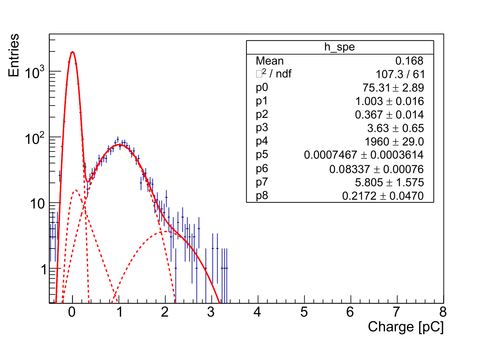
Fig. 14 SPE histogram at 3.7V control voltage
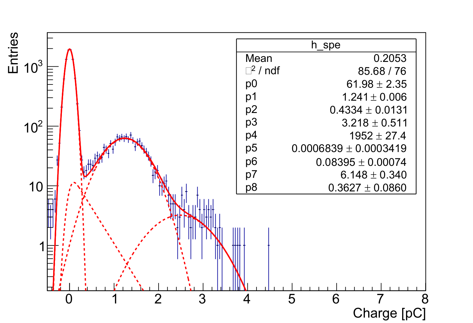
Fig. 15 SPE histogram at 3.8V control voltage
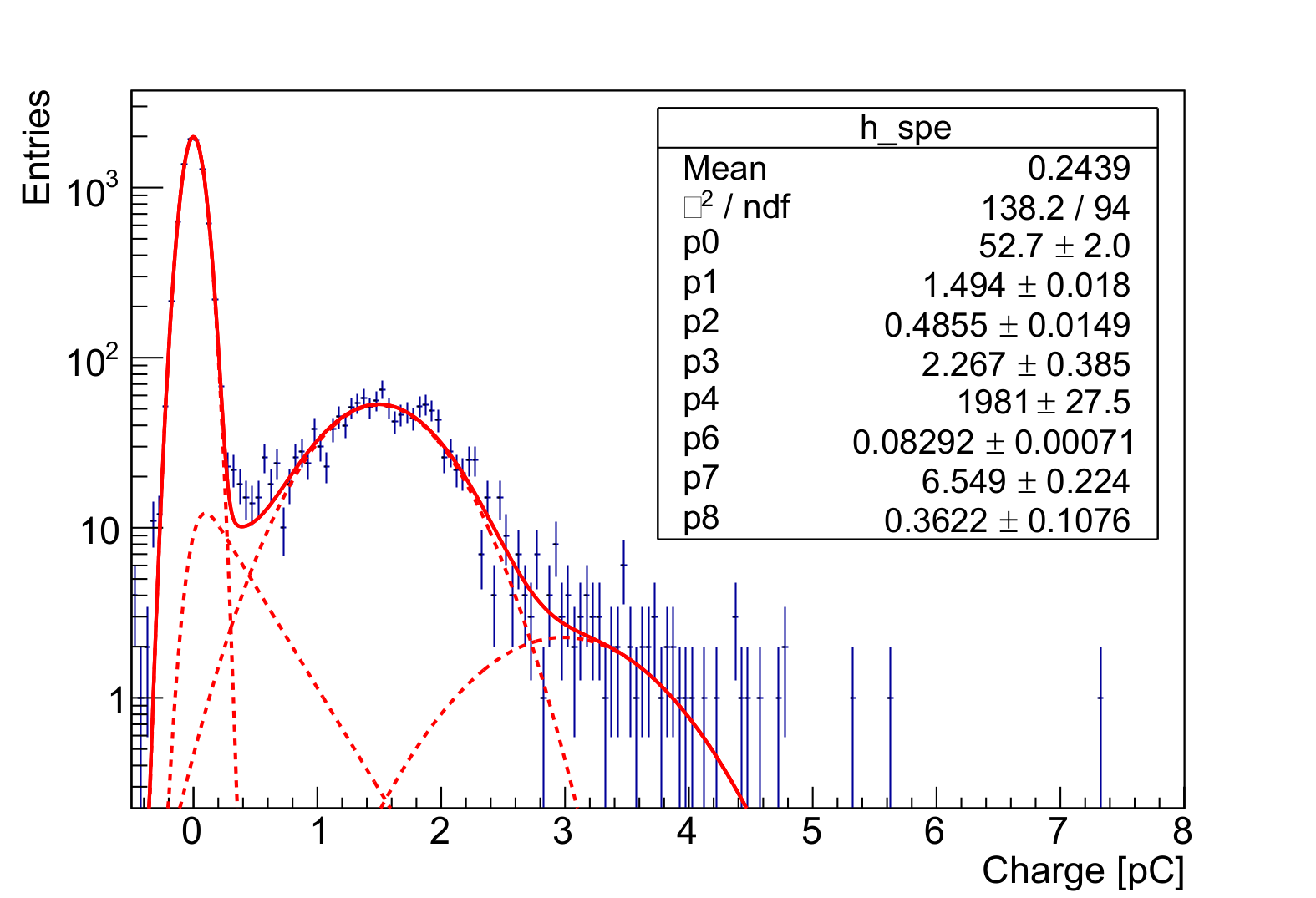
Fig. 16 SPE histogram at 3.9V control voltage
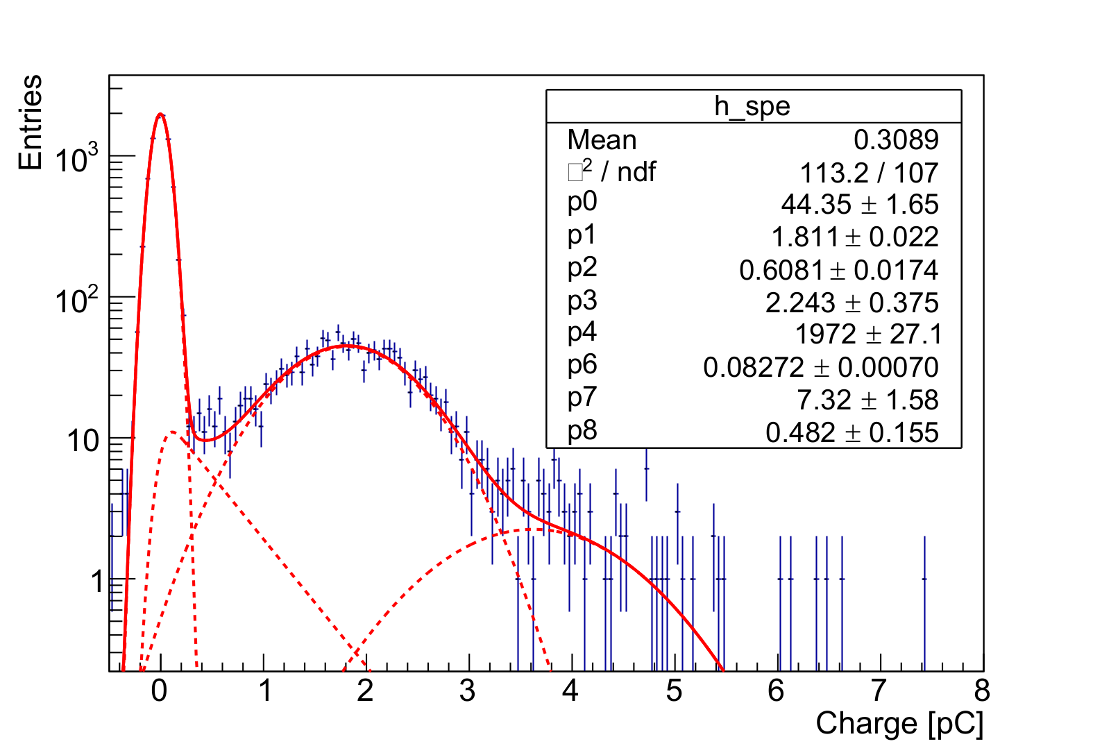
Fig. 17 SPE histogram at 4.0V control voltage
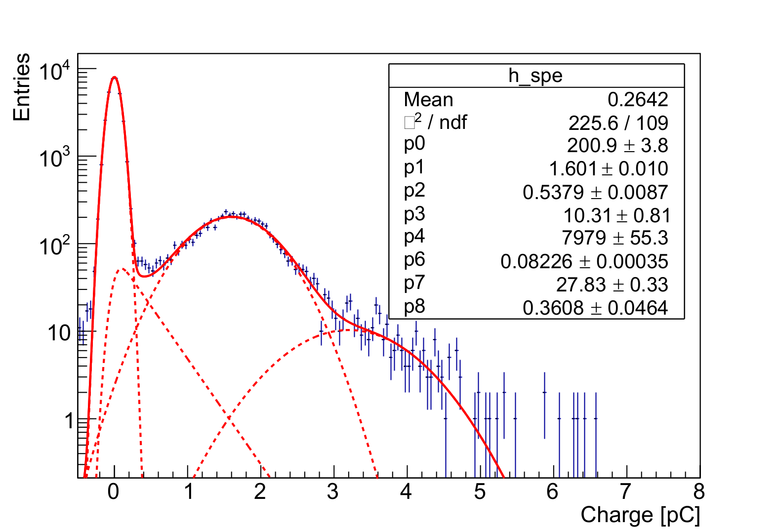
Fig. 18 SPE histogram at 3.93V control voltage with 4x the entries
Replace {pmtname} with the PMT name you gave the measurement in the notebook, replace {scan_point_value} with the value of one scan point:
python run.py {pmtname} {scan_point_value}V
Check the constructed SPE histogram for sanity, then go on to make the gain curve by running the following command:
python get_gain_curve.py {pmtname} {lv_value_0} {lv_value_1} {lv_value_2} {lv_value_3}
Again, check the constructed plots for sanity and write down the given optimal control voltage value.
Show/Hide example gaincurve
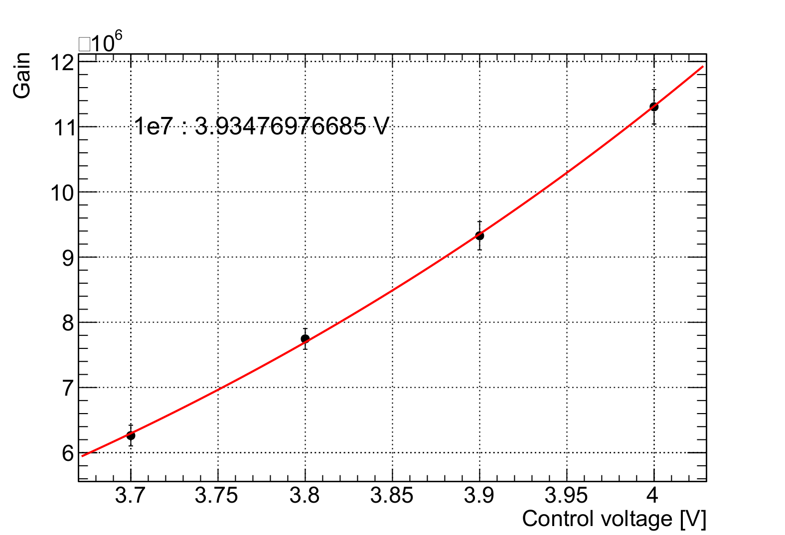
Fig. 19 Example gain curve used to determine the control voltage for 1E7 gain
Afterwards, run the second part of the notebook with the control voltage set to the extracted value.
The extraction of SPE spectrum parameters is done inside the tools/ subdirectory. Read the README for all commands.
Show/Hide example plots
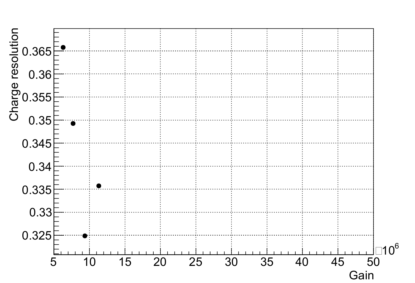
Fig. 20 Example charge resolution plot
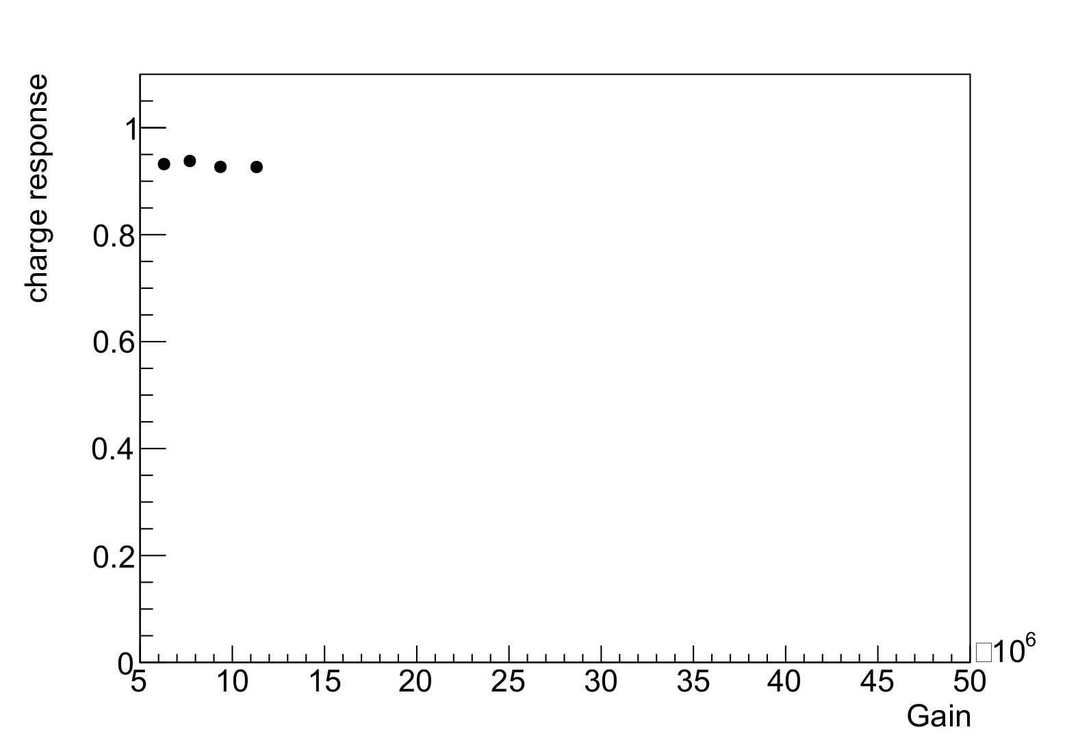
Fig. 21 Example charge response plot
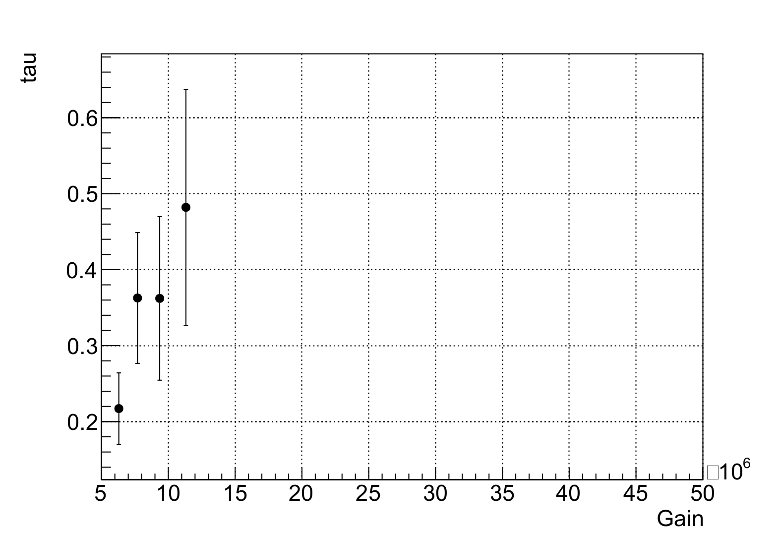
Fig. 22 Example tau plot