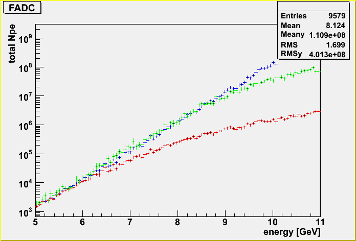
The purpose is to investigate the systematic difference between the K-function (parameterized function for the bulk tables) and the lightsaber tables (based on layered tables), and to reveal the systematic difference between bulk and layered tables.
Actually, similar study was already done by Sean. (See also this page.)
Here, I actually like to investigate the outcome from the difference of the PDFs, namely total Npe detected by all detectors from an EHE track.
I made a simple class to make ATWD and FADC waveforms from the PDFs. Summing up all the p.e's from a muon track, I get the total Npe.
I input muons randomly for a case, and fix the geometry for a case.

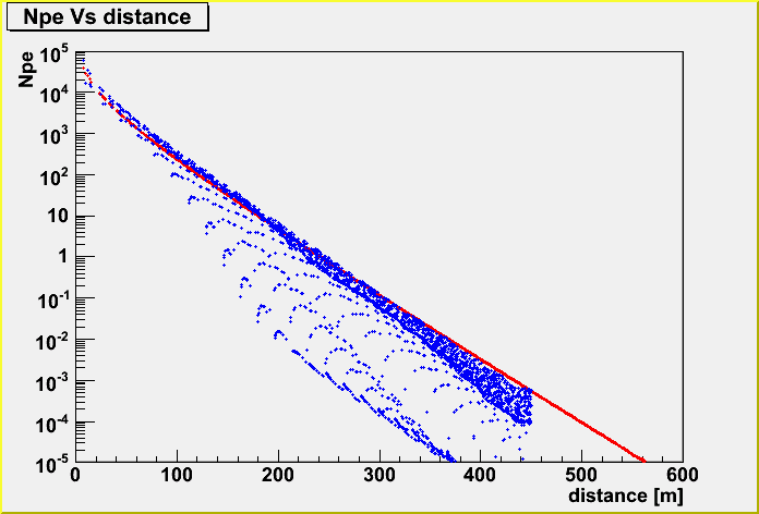
You see the Npe Vs distance relation above. The red is K-function and the blue is lightsaber. The input parent muon energy is 10^7 GeV, and the geometry is fixed (horizontal, going through the center of the IceCube detector).
You see clearly the layered effect, I think. (I will investigate this issue more soon.)
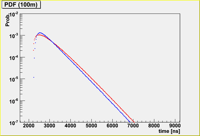
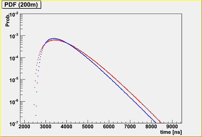
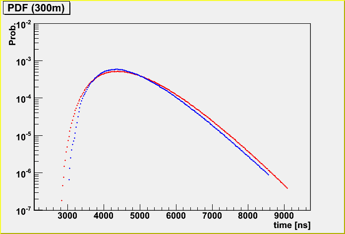
I also checked the PDF difference.
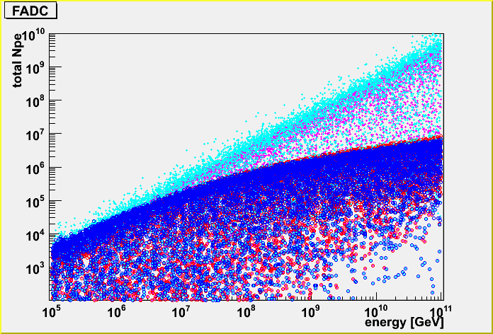
Firstly, fixed geometry (horizontal, going through the center of the IceCube detector). (The energy is randomized.)
The light blue is K-function and the blue is the case taking care of the detector dynamic range, and the pink is lightsaber tables without the dynamic range and the red is with dynamic range.
I found that thre is difference in amplitude between K-function and photonics tables in the parameterization. See the first plot of this.
So, I ignore OMs near to a tack within 10 m. Now the correlation between K-function and lightsaber tables becomes better. You can see it below with more statistics.
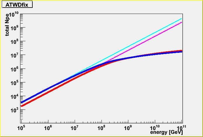
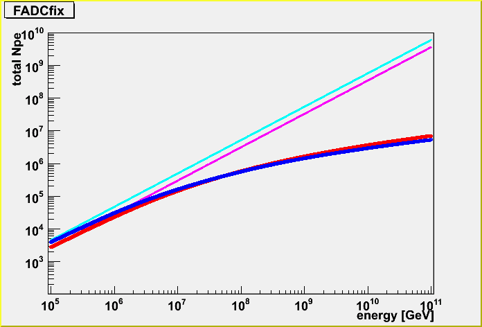
Randomized geometry case.
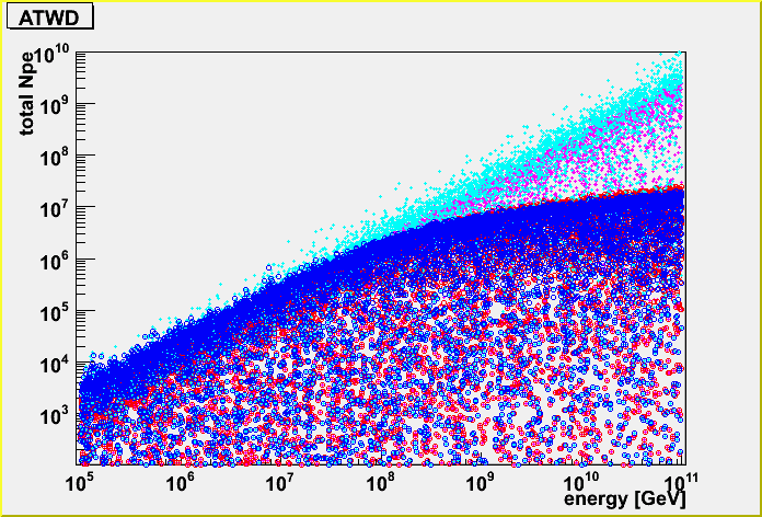
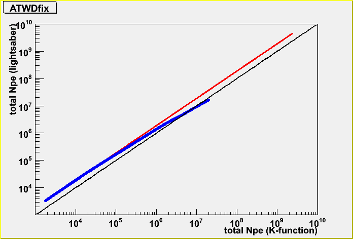
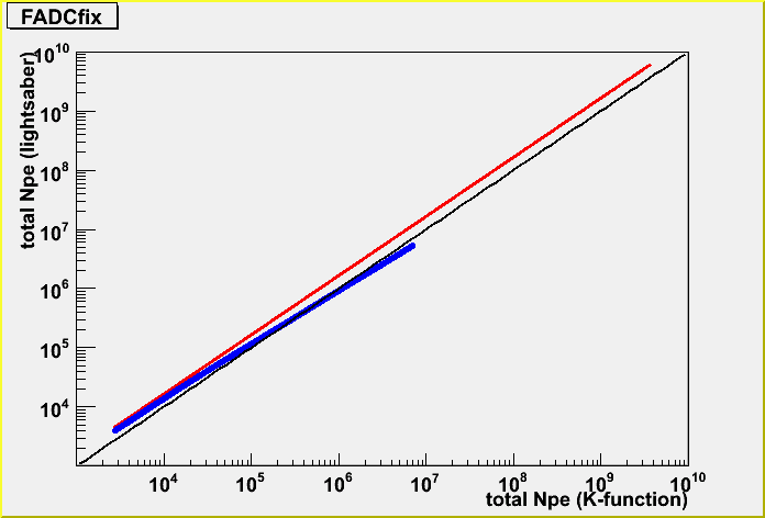
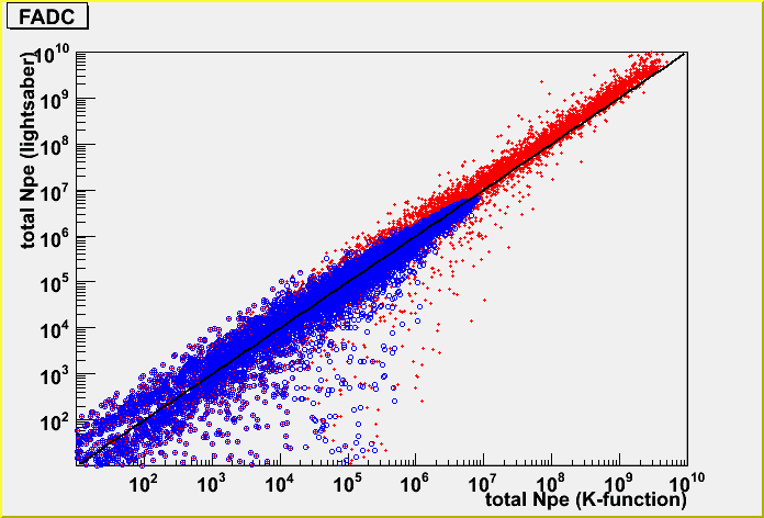
I took the correlation for the fixed geometry case.
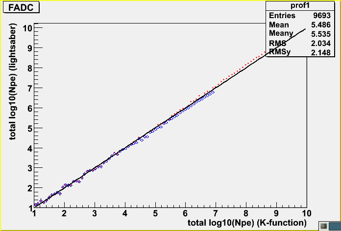
The red is without dynamic range, and the blue is with dynamic range. I simply add the y=x function for the reference.
and, randomized geometry case.
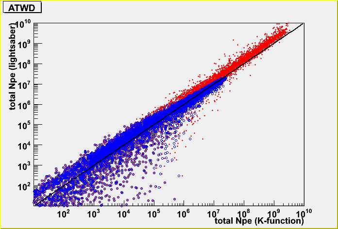
and, the profile for the randomized case.
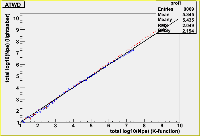
The difference between K-function and lightsaber tables
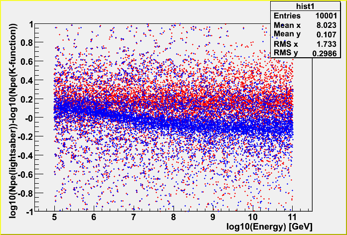

The large difference comes from track far from the center of the detector.
I guess this is because the lightsaber tables take into account the OM position with respect to a track, and K-function doesn't. I will investigate this more, too. (See the first plot on this page, too.)
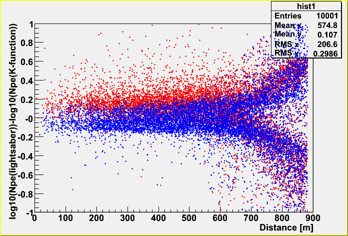
After the distance cut (dist<600m)
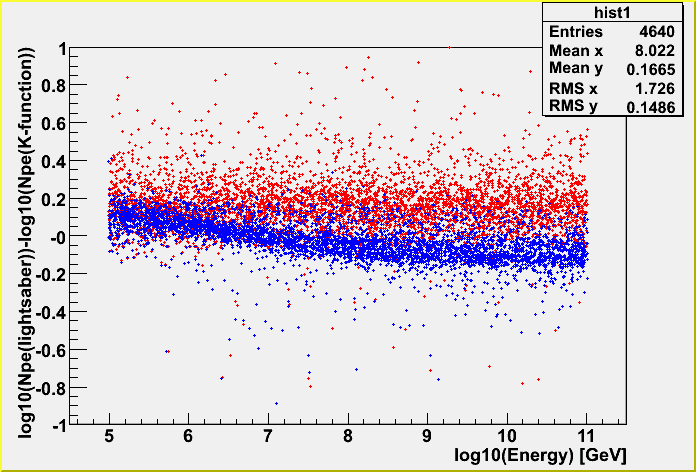
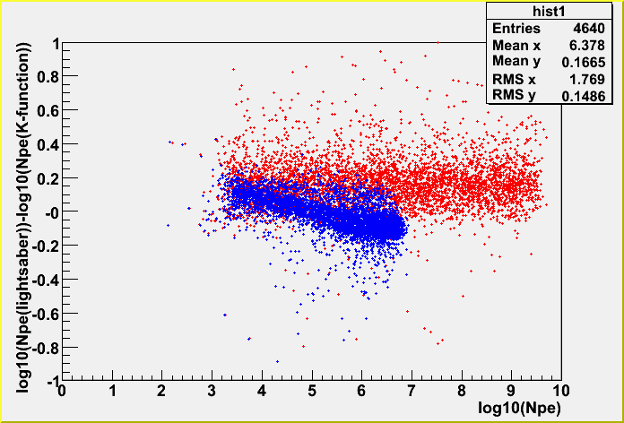
Histogram of the difference (with the distance cut) (If no distance cut, the distribution has a tail, but the rms doesn't change so much.)
10^5-6 GeV
Black: no dynamic range
Blue: with dynamic range
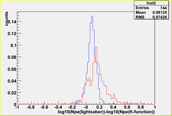
10^7-8 GeV
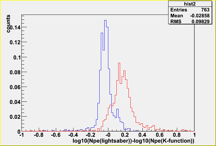
10^9-10 GeV
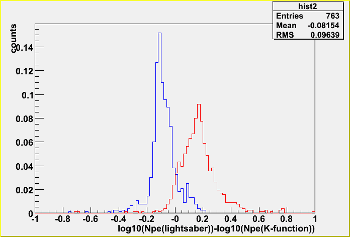
The spread is not so big. It's ~25%. So, as far as a track is inside the detector the difference between the layered and bulk tables in total Npe is this level, but not for an outer track.
There is a systematic shift, and this shift appears to be only for the case where the dynamic range is taken into account. This is because the lightsaber tables tend to give higher Npe in the waveform. (Remember the previous plots that show waveforms.)
At last, I show again the correlation plot between the K-function and the layered tables with the distance cut.

Some updates
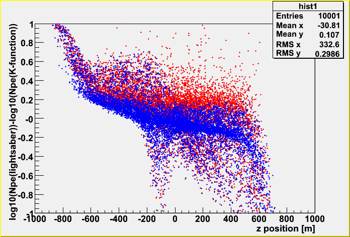
incident Z position dependence. (Z position at incident position around the 880 m radius.)
This plot mainly shows that K-function doesn't take into accout the track position with regards to DOM position. You may see some layered effects. Blue: with dynamic range, Red: without.
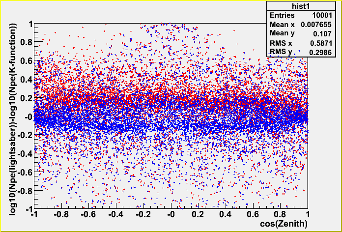
incident zenith angle dependence.
There is not so much effect of the zenith angle.
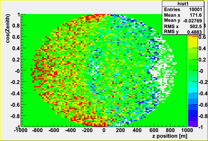
Two dimensional plots showing the dependence of z position and zenith angle.
The general trend is that when the track starts from down (z: negative) the lightsaber tables give more lights than K-function. You see some inveted region around the center position of the detector due to the layered tables effect.
I also checked the consistency between the K-function and juliet MC data.
Here is the profile.
Pink: K-function without dynamic range
Red: K-function with dynamic range
Green: juliet MC
In order to get the better agreement, I put a time-window for the MC hits of juliet MC data, and the distance cut for the near OM to a track is also applied.
