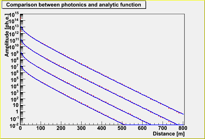
I got the amplitude distribution and time PDF for an EHE muon by convolution of many cascades using the Photonics tables (v1.5). I put many fixed energy cascades every ~2 m along a muon track according to my last study.
To get the parameterized function of the amplitude distribution, I fitted the distribution.
The function is expressed such as 44.55*E*dist^-0.80*exp(-3.364*10^-2*dist) (E in GeV). Be careful that, here, E is NOT the primary energy of a muon, BUT average cascade energy along the track (average energy loss from an EHE muon) in GeV. (Sorry about this confusion!) In order to get the parent energy, we should use the following equation from my last study.
[Energy loss in a cascade] = (-125.2+-349.7)+(6.214+-2.198)*10^{-4}*[Initial Energy].
[Energy loss in a cascade] = (4.486+-4.896)*10^-4*[Initial Energy]^(1.0204+-0.0434).
The dist is distance from a muon to a detector.
You can see the distribution (red) and the parameterized function (blue). The energies of average energy loss in a cascade are 10^6, 10^8, 10^10 and 10^12 GeV from below. The parameterized function express the distribution well except at 0 m.
To get the parameterized function of the time PDF, I fitted the distribution.
I fitted it with a function form of a0*t^a2*exp(-a1*t) for each distance.
The parameter of a0, a1 and a2 also depends on the distance as you can see the dependence in figures below.
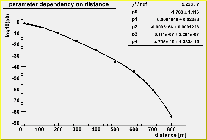
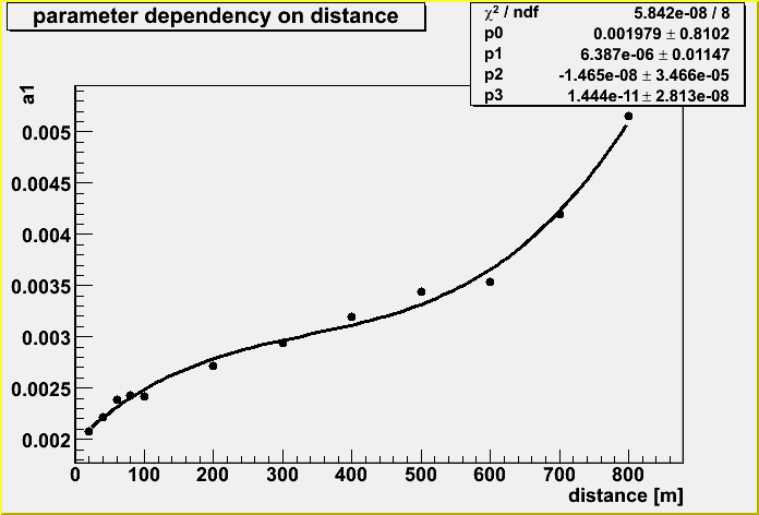
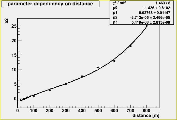
The parameters are also fitted as below;
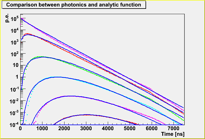
I plotted the time PDF for an EHE muon derived from convolution of Photonics cascade tables, and the derived parameterized functions. The blue lines are the parameterized functions, and other colors are for the convolution of the Photonics cascade tables. The distance is 50, 100, 200, 300, 400, 500, 600, 700 and 800 m from left side of the figure.
(The probability is per ns, although I plotted the PDF every 50 ns for an EHE muon distribution derived from the Photonics.)
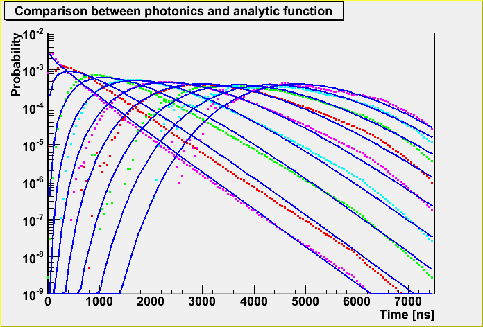
There is some deviation for 100 and 200 m between the distribution and the function.
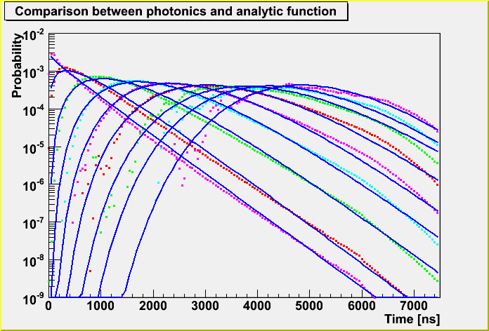
In order to get better fit, I used higher order of polinominal function to express the a1 and a2 parameters.
With these correction, we can express the distribution better as you can see the plot below.
However, there is a bad thing for this correction.
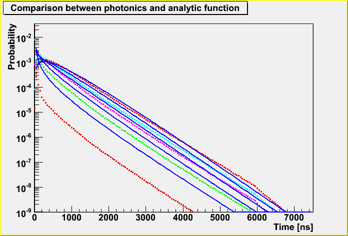
Now, we can not express the distribution for the shorter distances as below. The distances are 10, 30, 50, 70 and 90 m from the left.
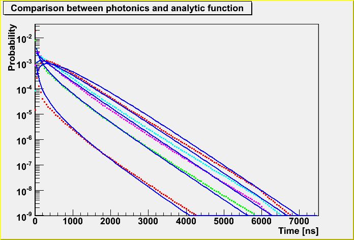
The parameterized function was such as below without the higher order correction, which more or less express the distributions.
That's why I took the lower order parameterization for a1 and a2 parameter that have some problem to express middle range (100 and 200 m) at first.
So, probably we can use the higher order correction to express the shorter distacne, and lower order for higher distance. The transition occures at around 30-40 m.
From below, I discribe the detail. Well, actually the shape of the function with the higher order correction is ok to express the shorter distances. The real problem is the normalization. As you may notice, the normalization factor is inside the a0 parameter, but it's deviate a lot from 10^-90 to ~1 (90 order of magnitude!). So, I made a re-normalization such that the integral of the function becomes 1.
However, for the shorter distances the parameter of a2 becomes negative, meaning that the distribution has a singularity at 0 ns. So, the re-normalization doesn't work well. Well, I made a trick to avoid this singularity. It's just to integral the function from a small offest (10^-3) not from 0. You may think we can adjust the normalization factor by changing the offset, but we can't freely change the value because of the limitation of the ROOT.
You see the PDF distribution weighted by the amplitude corresponded to the distance. This will be the distribution what we will get in ATWD or FADC data.
The plot below is the distribution for 10^8 GeV energy loss in a cascade, so the primary energy of an EHE muon is about 2x10^11 GeV, which will be a bit high energy events from the expected GZK signal. The distributions correspond to 50, 100, 200, 300, 400 and 500 m from the top. From this plot we will get p.e. signals up to ~200 m. We can also see that we will have a saturation for the near distance. From this plot, we can see probably the ATWD will not be useful at all up to ~50 m in this case.
Notice that the distribution scales to the energy.
Here, the blue lines are the parameterized function with the higher order correction, and they seem to be quite OK.