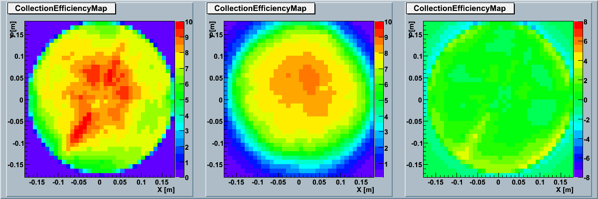
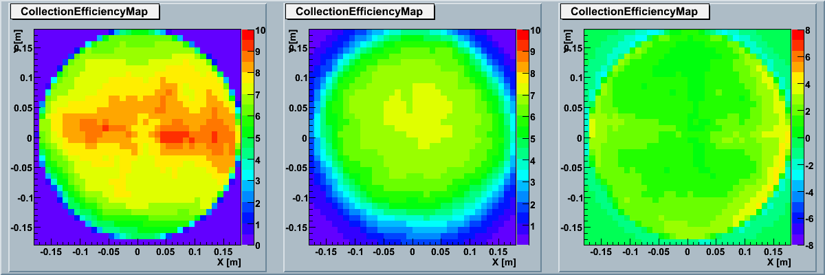
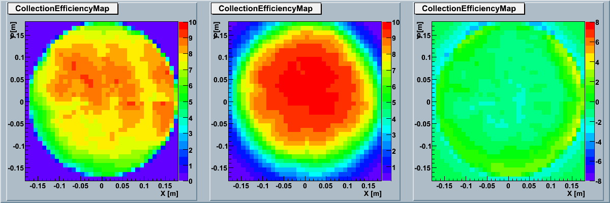
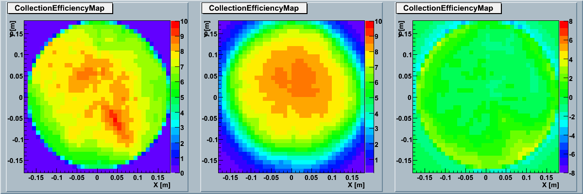
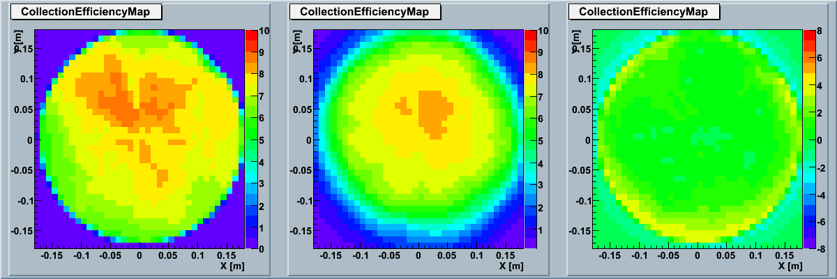
The 2005 Golden PMTs have a trend that the QE measured by Chiba appears approximately 15% higher than that indpendently measured by HAMAMATSU using the DC light source. To take into account this difference, the present analysis are divided by the two independent categories - one uses the Chiba numbers while another uses the Hamamatsu values. Then we decide which case appears more reasonable judged by the amount of the correction it needs to be consistent with the GDOM calibration data.
In conclusion, the ROMEO using the HAMAMATSU QE numbers with shifting
the wavelength of -5 nm in the GEANT4-based glass+gel acceptance table
describes the GDOM calibration data in the best manner. We use
this "3.38nm wavelength shift recipe" to the
FY 2006 GDOMs analysis
as well to see if it also works or not.
Analysis method
The ROMEO simulatrion is performed with the configuration
following the condition of the GDOM calibraion measurement at Chiba
such as light intensity and beam size of the LED. The simulated data
describes the absolute detection efficiencies as a function
of the location on the DOM sphere. Then it is compared
with the 2D DOM scan data with normalization determined by
the absolute calibration. Then we shift the wavelength of
the internal ROMEO's glass+gel acceptance table
and repeat the same procedure. The amount of the wavelength shift
to give the best agreement between the simulation and the data
is determined.
Description of the table
PMT QE at 337nm. By default it should be Chiba measurement value.
DOM QE at 337nm measured by Chiba.It includs systematic error about 8%.
mean of difference from GDOM Efficiency (data) AFTER compensation
[diff]:The histogram of QE(sim-data)[%].
[0~168deg][180~348deg]: Figs of AbsoluteQE[%] vs distance on cathode for each azimuth axsis.
Shifted length of Wavelength
Acceptance (of glass+gel) x-axis (wavelength axis)->corresponds uncertainty of transparency
| PMT | Chiba measurement | Hamamatsu measurement |
| TA1052 | 20.74% | 17.40% |
| TA1059 | 20.69% | 16.25% |
| TA1062 | 20.79% | 17.95% |
| TA1069 | 20.43% | 16.79% |
| TA1167 | 19.71% | 15.89% |
| PMTName | QE337nm[%] | DOM data[%] | Before Compensation | correction | After Compensation | ||||
|---|---|---|---|---|---|---|---|---|---|
| sim-data[%] | sim-data /data[%] |
fig | shift x[nm] | sim-data[%] | sim-data /data[%] |
fig | |||
| TA1052 | 20.74 | 8.29 | 3.053 | 36.8 | [diff] [0~168deg] [180~348deg] | -8.5 | 0.005699 | 0.07 | [diff] [0~168deg] [180~348deg] |
| TA1059 | 20.69 | 7.03 | 3.874 | 55.1 | [diff] [0~168deg] [180~348deg] | -10.0 | 0.2625 | 3.7 | [diff] [0~168deg] [180~348deg] |
| TA1062 | 20.79 | 9.66 | 1.702 | 17.6 | [diff] [0~168deg] [180~348deg] | -5.1 | 0.009393 | 0.10 | [diff] [0~168deg] [180~348deg] |
| TA1069 | 20.43 | 8.34 | 2.489 | 29.8 | [diff] [0~168deg] [180~348deg] | -7.2 | 0.05923 | 0.71 | [diff] [0~168deg] [180~348deg] |
| TA1167 | 19.71 | 7.74 | 2.878 | 37.2 | [diff] [0~168deg] [180~348deg] | -8.4 | -0.0579 | 0.75 | [diff] [0~168deg] [180~348deg] |
| average | 20.47 | 8.21 | 2.80 | 34.1 | [diff] [0~168deg] [180~348deg] | - | 0.056 | 0.68 | [diff] [0~168deg] [180~348deg] |
| PMTName | QE337nm[%] | DOM data[%] | Before Compensation | correction | After Compensation | ||||
|---|---|---|---|---|---|---|---|---|---|
| sim-data[%] | sim-data /data[%] |
fig | shift x[nm] | sim-data[%] | sim-data /data[%] |
fig | TA1052 | 20.74 | 8.29 | 3.053 | 36.8 | [diff] [0~168deg] [180~348deg] | -7.84 | 0.2963 | 3.6 | [diff] [0~168deg] [180~348deg] |
| TA1059 | 20.69 | 7.03 | 3.874 | 55.1 | [diff] [0~168deg] [180~348deg] | -7.84 | 1.153 | 25.0 | [diff] [0~168deg] [180~348deg] |
| TA1062 | 20.79 | 9.66 | 1.702 | 17.6 | [diff] [0~168deg] [180~348deg] | -7.84 | -1.082 | 11.2 | [diff] [0~168deg] [180~348deg] |
| TA1069 | 20.43 | 8.34 | 2.489 | 37.2 | [diff] [0~168deg] [180~348deg] | -7.84 | -0.1944 | 2.3 | [diff] [0~168deg] [180~348deg] |
| TA1167 | 19.71 | 7.74 | 2.878 | 37.2 | [diff] [0~168deg] [180~348deg] | -7.84 | 0.1793 | 2.3 | [diff] [0~168deg] [180~348deg] |
| average | 20.47 | 8.21 | 2.80 | 34.1 | [diff] [0~168deg] [180~348deg] | -7.84 | 0.07 | 0.86 | [diff] [0~168deg] [180~348deg] |
| PMTname/DOMname | wavelength | After Compensation |
| TA1052/Shino_Inuzuka | 337nm |  |
| TA1059/Shinbei_Inue | 337nm |  |
| TA1062/Kobungo_Inuta | 337nm |  |
| TA1069/Sosetsu_Inuyama | 337nm |  |
| TA1167/Genpachi_Inukai | 337nm |  |
| PMTName | QE337nm | DOM data | Before Compensation | correction | After Compensation | ||||
|---|---|---|---|---|---|---|---|---|---|
| sim-data[%] | sim-data /data[%] |
fig | shift x[nm] | sim-data[%] | sim-data /data[%] |
fig | |||
| TA1052 | 17.40 | 8.29 | 1.284 | 15.5 | [diff] [0~168deg] [180~348deg] | -4.6 | 0.05034 | 0.61 | [diff] [0~168deg] [180~348deg] |
| TA1059 | 16.25 | 7.03 | 1.582 | 22.5 | [diff] [0~168deg] [180~348deg] | -5.9 | 0.04774 | 0.68 | [diff] [0~168deg] [180~348deg] |
| TA1062 | 17.95 | 9.66 | 0.1795 | 1.9 | [diff] [0~168deg] [180~348deg] | -0.7 | 0.04083 | 0.42 | [diff] [0~168deg] [180~348deg] |
| TA1069 | 16.79 | 8.34 | 0.5921 | 7.1 | [diff] [0~168deg] [180~348deg] | -2.4 | 0.05222 | 0.63 | [diff] [0~168deg] [180~348deg] |
| TA1167 | 15.89 | 7.74 | 0.8054 | 10.4 | [diff] [0~168deg] [180~348deg] | -3.3 | 0.02777 | 0.36 | [diff] [0~168deg] [180~348deg] |
| average | 16.9 | 8.21 | 0.889 | 10.8 | [diff] [0~168deg] [180~348deg] | - | 0.044 | 0.53 | [diff] [0~168deg] [180~348deg] |
| PMTName | QE337nm[%] | DOM data[%] | Before Compensation | correction | After Compensation | ||||
|---|---|---|---|---|---|---|---|---|---|
| sim-data[%] | sim-data /data[%] |
fig | shift x[nm] | sim-data[%] | sim-data /data[%] |
fig | |||
| TA1052 | 17.40 | 8.29 | 1.284 | 15.5 | [diff] [0~168deg] [180~348deg] | -3.38 | 0.4146 | 5.0 | [diff] [0~168deg] [180~348deg] |
| TA1059 | 16.25 | 7.03 | 1.582 | 22.5 | [diff] [0~168deg] [180~348deg] | -3.38 | 0.7627 | 10.8 | [diff] [0~168deg] [180~348deg] |
| TA1062 | 17.95 | 9.66 | 0.1795 | 1.9 | [diff] [0~168deg] [180~348deg] | -3.38 | -0.7096 | 7.3 | [diff] [0~168deg] [180~348deg] |
| TA1069 | 16.79 | 8.34 | 0.5921 | 7.1 | [diff] [0~168deg] [180~348deg] | -3.38 | -0.2092 | 2.5 | [diff] [0~168deg] [180~348deg] |
| TA1167 | 15.89 | 7.74 | 0.8054 | 10.4 | [diff] [0~168deg] [180~348deg] | -3.38 | 0.002462 | 0.03 | [diff] [0~168deg] [180~348deg] |
| average | 16.9 | 8.21 | 0.889 | 10.8 | [diff] [0~168deg] [180~348deg] | -3.38 | 0.052 | 0.64 | [diff] [0~168deg] [180~348deg] |
| PMTname/DOMname | wavelength | After Compensation |
| TA1052/Shino_Inuzuka | 337nm | 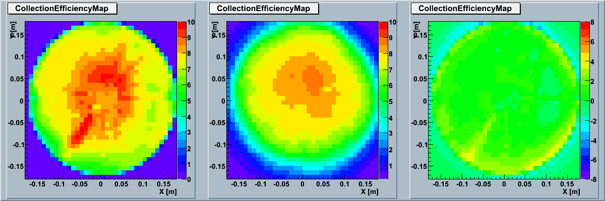 |
| TA1059/Shinbei_Inue | 337nm | 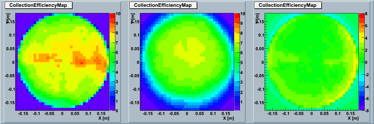 |
| TA1062/Kobungo_Inuta | 337nm | 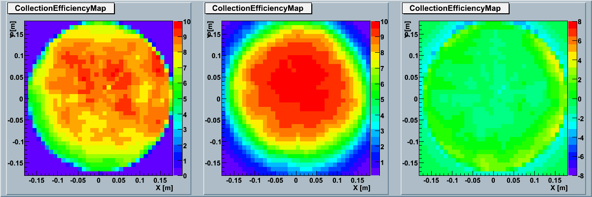 |
| TA1069/Sosetsu_Inuyama | 337nm | 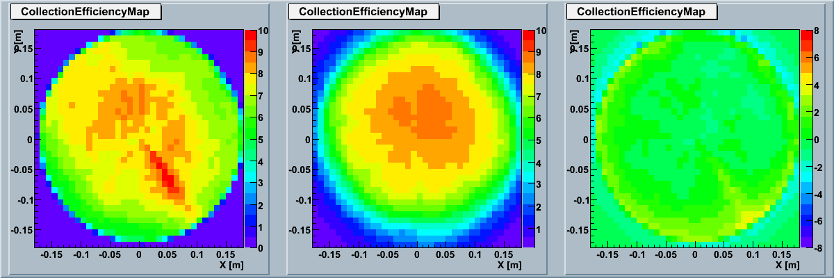 |
| TA1167/Genpachi_Inukai | 337nm | 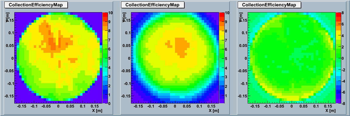 |