DEgg 2D Photon Detection Efficiency Scan
This page summarizes the measurement procedure and analysis necessary for DEgg half 2D scans of the absolute photon detection efficiency [PDE] map.
The setup used for this measurement is the 2D scan box in the darklab in combination with the reference line setup in the laser darkbox.
The strategy for this measurement is to count detected photons at the DEgg dependent on the illuminated spot on the photocathode and compare it to the number of detected photons at a reference PMT, which has been absolutely calibrated by Hamamatsu before.
This measurement requires some calibrations of the beamline, gain of the DEgg half and reference PMT, and the positional dependence of the DEgg gain on the photocathode.
We start with calibration runs, then move on to the PDE scan.
Calibrations
Beamline Calibration
Rationale
The goal of this calibration is to determine the number of photons that arrive at the end of the signal line per photon that arrives at the end of the reference line. This includes effects of the laser alignment, beamsplitter efficiency, and coupling into the optical fibers.
The strategy here is to use the reference PMT both at the end of the signal line as well as the reference line. The mounting of the reference PMT at the signal line end requires a 3D printed holder, which attaches to the driveable fiber end mount. Figure Fig. 37 shows the printed holder.
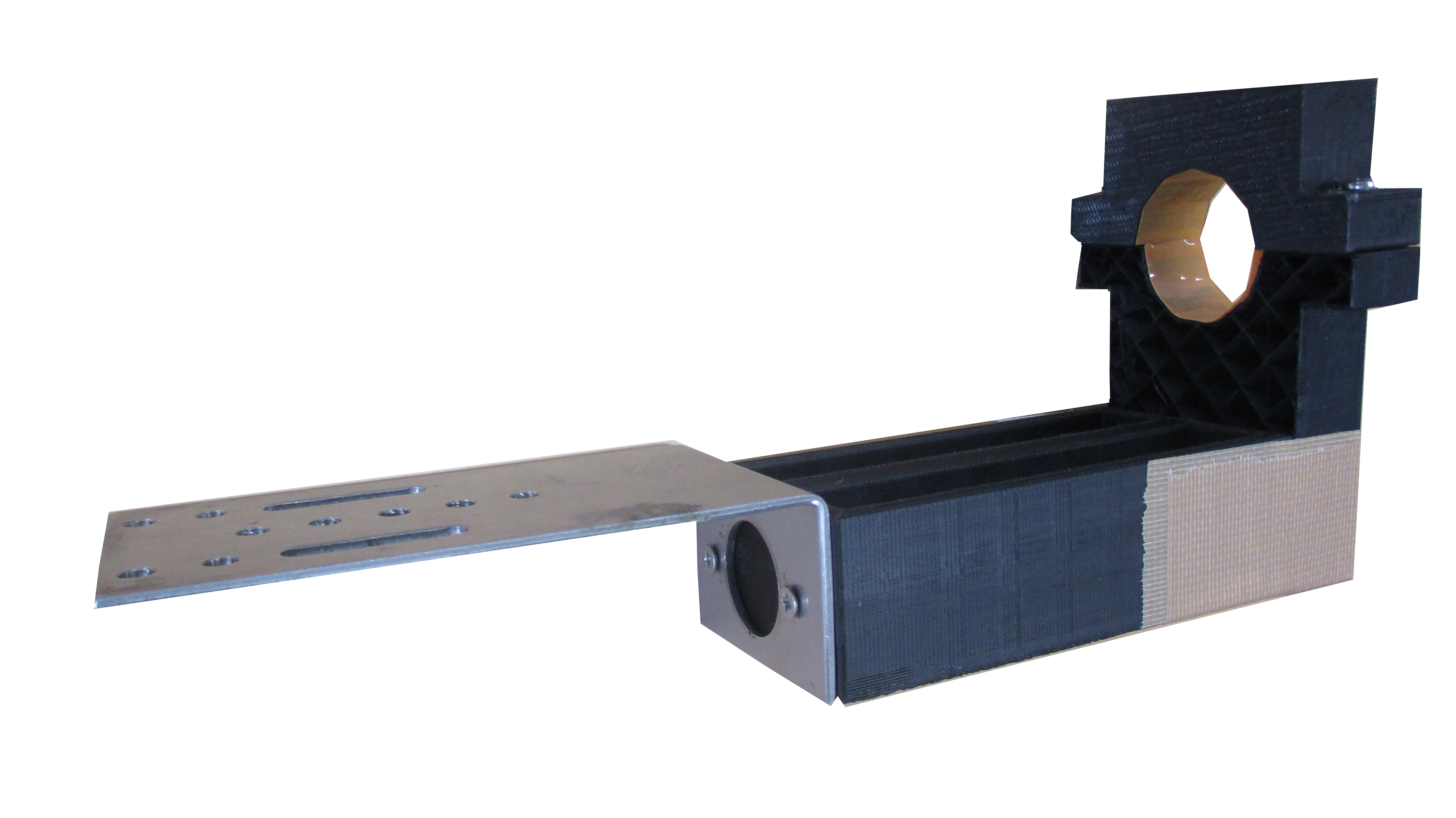
Fig. 37 3D printed mount for the reference PMT for the 2D scan box.
DAQ settings
The oscilloscope used is the Rhode&Schwarz RTO1044 next to ratafia, the laser trigger line is connected to channel 4, the signal line readout is connected to channel 3, the reference line readout is connected to channel 2.
The trigger is to be set in normal mode to the laser trigger signal on the falling flank.
This measurement is to be done at MPE level. Make sure, that the filter in the laser darkbox is set to 1% and the waveform peak voltage is roughly at -600mV. The laser frequency should not exceed 100Hz.
Only the reference PMT is used for this measurement. Since we want to compare the response at both fiber ends, the high voltage for both runs needs to be set to the same value of -1500V.
Running the DAQ
The data acquisition is controlled by a jupyter notebook. It is located at:
/home/icecube/lasse/notebooks/beamline_calibration/beamline_calibration.ipynb
It records 10000 waveforms. You need to run it twice, once with the reference PMT mounted in the laser darkbox, and once with it mounted in the 2D scan box. Make sure to name the storage directory for the reference run with ‘reference_line’ and ‘signal_line’ respectively.
Analysis of raw data
The analysis script is called count_pulses.py. It is located at:
/home/icecube/lasse/analysis/beamline_calibration/mpe_beamline_calib.py
To get an overview of its functionality, run:
python3 mpe_beamline_calib.py --help
Since the gain of the reference PMT is the same for both runs, this script integrates the waveforms in the given gates. Please check, that these make sense, use the –plot_n_waveforms option for that and adjust the gates accordingly. Finally, the script divides the charges seen in both lines, which are fully correlated with the number of arrived photons, and spits out the beamline calibration factor.
Scan Box Uniformity
Rationale
The goal of this calibration is two assess how dependent the light yield at the end of the signal line fiber is on the scan position.
This calibration is performed with the reference PMT mounted to the signal line end. The mount allows for full range of motion of the motors.
There is a caveat when trying to apply this calibration to scans with a DEgg half in the scan box. Any inhomogeneities that occur with the reference PMT in the scan box could come from reflections and edge effects, that can be substantially different, when the DEgg sits in the scan box.
This measurement does not need to be done for every DEgg.
DAQ settings
The oscilloscope used is the Rhode&Schwarz RTO1044 next to ratafia. Channel 4 is connected to the laser trigger output. The reference PMT is either connected to the signal line readout on channel 3 or to the reference line readout at channel 2. The oscilloscope should trigger on falling flanks on channel 4 in normal mode.
This calibration is done at SPE level. Make sure, that the filter in the laserbox is set to 0.1% and adjust the laser intensity such that the occupancy of the PMT is roughly at 10%. The laser pulse frequency should not exceed 100Hz.
The reference PMT is operated at -1500V.
Running the DAQ
The DAQ software lives in a jupyter notebook located at:
/home/icecube/lasse/notebooks/pmt_box_zenith_azimuth_calibration/pmt_box_calibration.ipynb
The notebook steers the motors and takes 1000 waveforms at each scan point.
Analysis
The analysis script lives in:
/home/icecube/lasse/analysis/pmt_box_zenith_azimuth/plot_zenith_azimuth_uniformity.py
A help message can be displayed by running the script with the –help flag.
It integrates all waveforms and counts how many have an integrated charge above a default threshold of 0.4pC. The number of these pulses is plotted as a function of zenith for all scanned azimuth slices as well as on a 2D polar plot.
Show/Hide some example plots
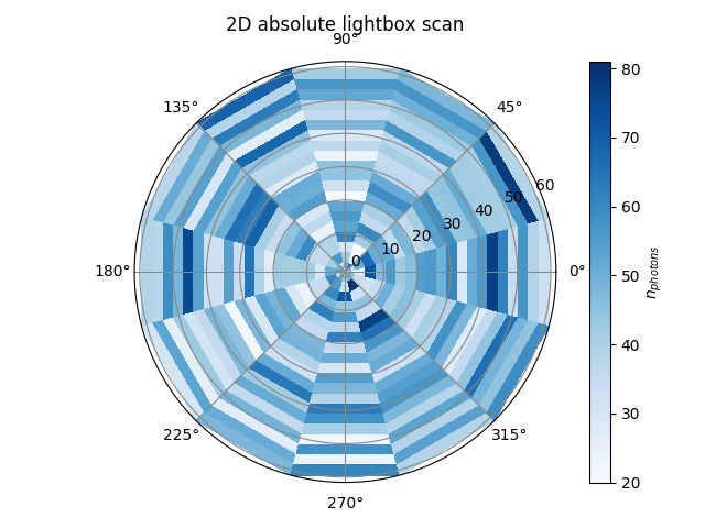
Fig. 38 2D Absolute Uniformity Map Of The Scan Box
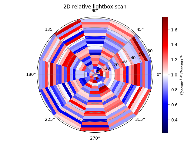
Fig. 39 2D Relative Uniformity Map Of The Scan Box
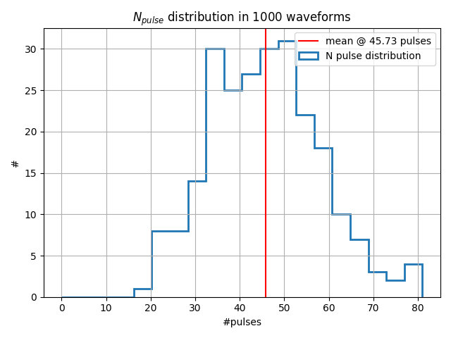
Fig. 40 Distribution Of Number Of SPE Pulses
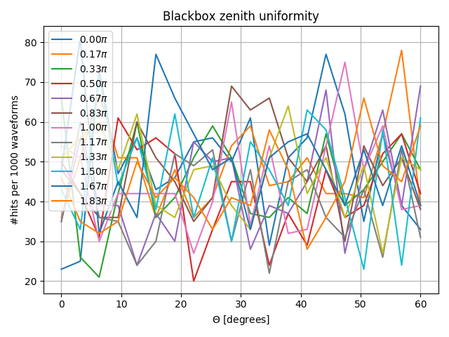
Fig. 41 Number Of Pulses vs. Zenith
Gain Calibration
Rationale
This calibration aims to measure the control voltage of the DEgg corresponding to a gain of 1E7 as well as to measure the gain of the reference PMT.
The gain of the DEgg and reference PMT are required for the 2D PDE scan, since it relies on photon counting at multiple PE level.
DAQ Settings
Use the Rhode&Schwarz RTO1044 next to ratafia. The measurement is done at SPE level. Set the laser intensity accordingly. Set the DEgg half into the holder inside the scan box and connect low voltage supply as well as the readout cabling to channel 3 of the oscilloscope.
The reference PMT is connected to channel 2 of the oscilloscope, the laser trigger signal is connected to channel 4. The oscilloscope trigger should be configured for falling flanks on the laser trigger signal in normal mode.
Running the DAQ
The measurement program is controlled by a jupyter notebook. It is located at:
/home/icecube/measurements/daq/notebooks/gain_calibration.ipynb
For the measurement of the correct control voltage, four points in voltage scattered around the value given by Hamamatsu are used to record 10000 waveforms with the laser illuminating the center of the cathode.
After determination of the correct control voltage, a measurement of the SPE spectrum with 40000 waveforms is done.
The reference PMT is operated at -1500V.
Analysis
The analysis script is located at:
/home/icecube/lasse/analysis/2d_gain_calibration/gain_vs_lv_scan.py
The usage of the script can be displayed by running the script with the –help flag.
The gains at each voltage setting are computed by a fit to the SPE spectrum constructed by integrating all waveforms. The optimal voltage setting is extracted from a fit to the measured gains.
The same script can be used to determine the gains of the DEgg at the inferred control voltage as well as for the reference PMT.
Show/Hide example plots
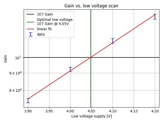
Fig. 42 Gain vs. low voltage scan of DEgg
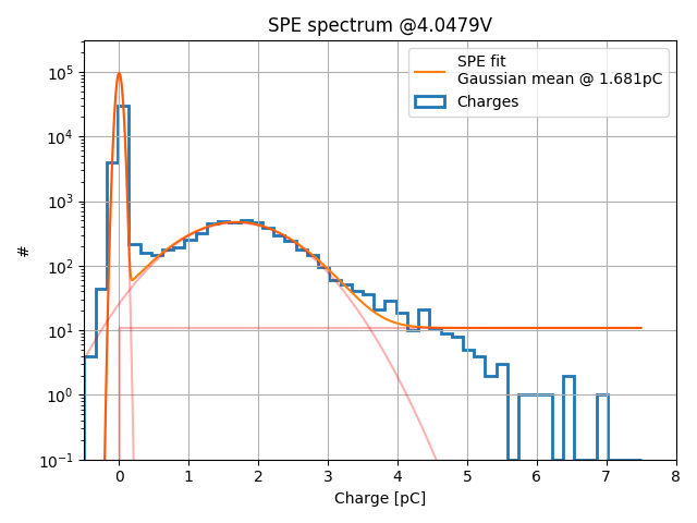
Fig. 43 SPE spectrum of DEgg at low voltage extracted from gain scan
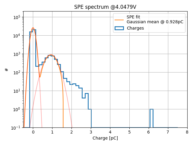
Fig. 44 SPE spectrum of reference PMT at -1500 V
DEgg 2D Gain Map
Additionally, a coarse 2D scan of the gain on the Cathode area of the DEgg is performed. The photocathode gain scan is done with 10000 waveforms at SPE level at each scan points.
Rationale
This calibration aims to evaluate the variation of the gain on the photocathode. Variations of the gain on the photocathode would lead to the same pattern in the photon-detection-efficiency scan.
DAQ Settings
The control voltage at the DEgg should be set to the one inferred to lead to a gain of 1E7. All other settings are the exact same as for the standard gain calibration.
Additionally, the Helmholtz Coils need to be activated for this measurement. The nominal voltage for the x-stage is 18 V, the nominal voltage for the y-stage is 12 V. The z-stage is not used for this measurement.
Running the DAQ
The DAQ is controlled by a jupyter notebook. It is located at:
/home/icecube/lasse/notebooks/2d_gain_scan/gain_calibration.ipynb
The notebook drives the motors of the scan box and record 10000 waveforms at each scan point.
Analysis
The analysis script is located at:
/home/icecube/lasse/analysis/2d_gain_calibration/make_gain_maps_2d.py
It can be executed with the –help flag to get an overview of the usage.
The script produces SPE spectra for each scan position and evaluates the position of the SPE peak for computing the gain.
A dictionary of gains and their errors is produced as well as plots showing the gain as function of zenith and 2D gain maps.
Show/Hide typical plots
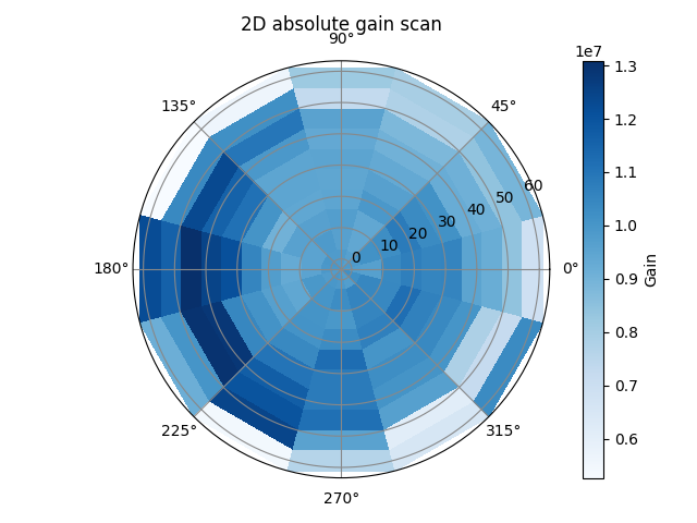
Fig. 45 2D absolute gain map
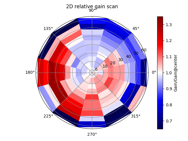
Fig. 46 2D relative gain map
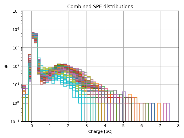
Fig. 47 Combined SPE distribution plot
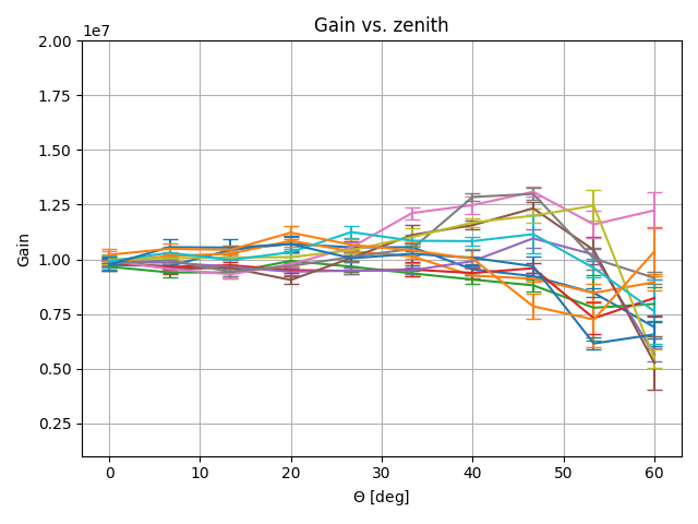
Fig. 48 Gain curves as function of zenith
DEgg 2D PDE Scan
Rationale
The 2D scan for determining the photon-detection-efficiency is done on MPE level. This keeps data consumption down, but makes a position dependent gain calibration necessary.
The idea here is to count the number of photons, that are detected at the DEgg half and compare it to the number of detected photons at the absolutely calibrated reference PMT.
DAQ Settings
Since this measurement is done at a level of ~40PE per pulse, the filters in the optical setup and the laser intensity need to be set accordingly.
The Rhode&Schwarz oscilloscpe RTO1044 next to ratafia oscilloscope is used. Channel 4 is connected to the laser trigger line, channel 3 is connected to the signal line, channel 2 is connected to the reference PMT. The trigger of the oscilloscope need to be configured on the laser trigger falling flank in normal mode.
The Helmholtz Coils need to be activated for this measurement. Set the x-stage voltage to 18 V, and the y-stage to 12 V.
Running the DAQ
The DAQ is controlled by a jupyter notebook, it is located at:
/home/icecube/lasse/notebooks/2d_mpe_pde_scan/2d_mpe_scan.ipynb
It records 200 waveforms on a fine azimuth, zenith grid for the DEgg as well as the reference PMT.
Analysis
Since this measurement produced a lot of data, we first integrate all waveforms and store the integrated charges in dictionary. The script that does that is:
/home/icecube/lasse/analysis/2d_mpe_absolute_pde/build_charge_dict.py
Afterwards, the absolute PDE at every scan point is computed with this equation:
That is implemented in this script, which can be evoked with the –help flag:
/home/icecube/lasse/analysis/2d_mpe_absolute_pde/mpe_absolute_pde_scan.py
The terms in the last fraction compare counted photons at the DEgg in some scan point to the counted photons seen at the reference PMT at the same time. It includes a correction with the position dependent gain of the DEgg. This is realized by either taking the gain at the nearest scan point from a specified 2D gain scan, or uses an interpolation on the gain map. The beamline factor compensates for differences in the beamline efficiencies. Finally, the PDE is computed by multiplying with the reference PMT PDE.
Show/Hide typical plots
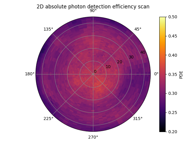
Fig. 49 DEgg 2D absolute PDE scan
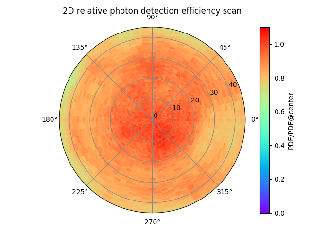
Fig. 50 DEgg 2D relative PDE scan
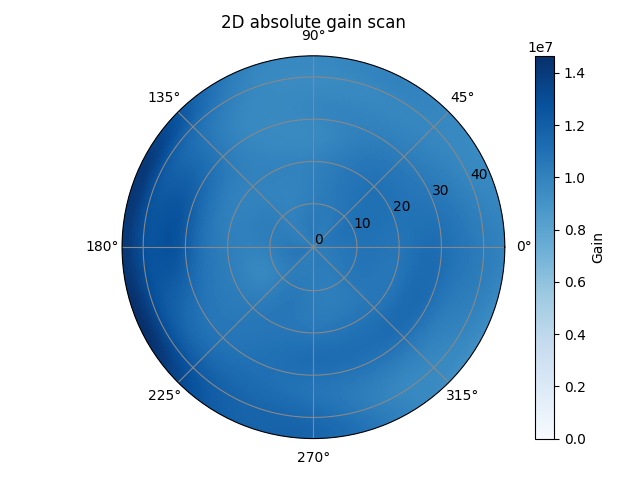
Fig. 51 DEgg 2D absolute Gain scan
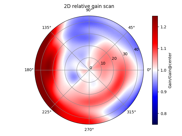
Fig. 52 DEgg 2D relative Gain scan
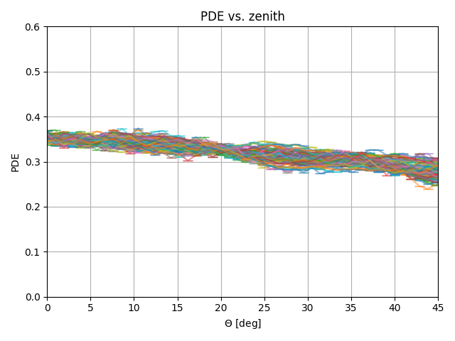
Fig. 53 PDE vs zenith plot
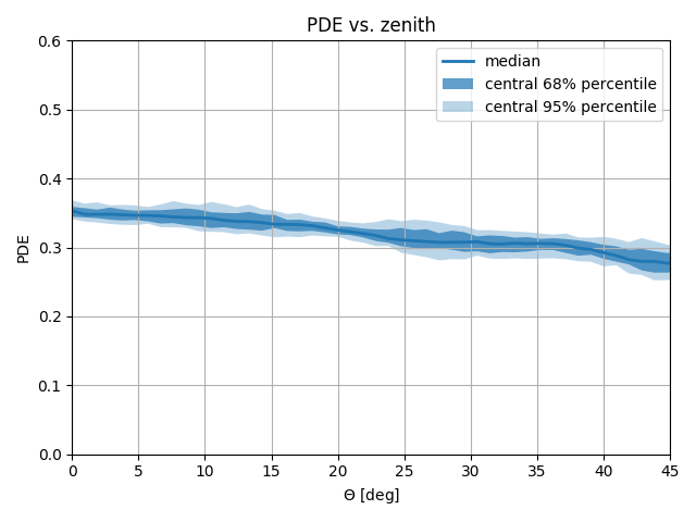
Fig. 54 PDE vs zenith band plot
Results
There are results for four D-Egg halves ready for download and playing around with. They are contained in .pckl files, which can be opened e.g. with the python pickle package. Each D-Egg half has a gain_dict_sq02xx.pckl and a pde_dict_sq02xx.pckl. Inside the gain_dict_sq02xx.pckl, you will find a python dictionary. It maps spherical coordinates to a tuple of [gain, gain_err], both values come from fits to the SPE peak. The keys are structured like this: (azimuth in rad, zenith in rad). The pde_dict_sqxx.pckl contains a similar python dictionary. The keys are structured in the same way, the values are single floats for the measured PDE. Find the files here:
gain_dict_sq0258.pckl pde_dict_sq0258.pckl
gain_dict_sq0287.pckl pde_dict_sq0287.pckl